Quality Control
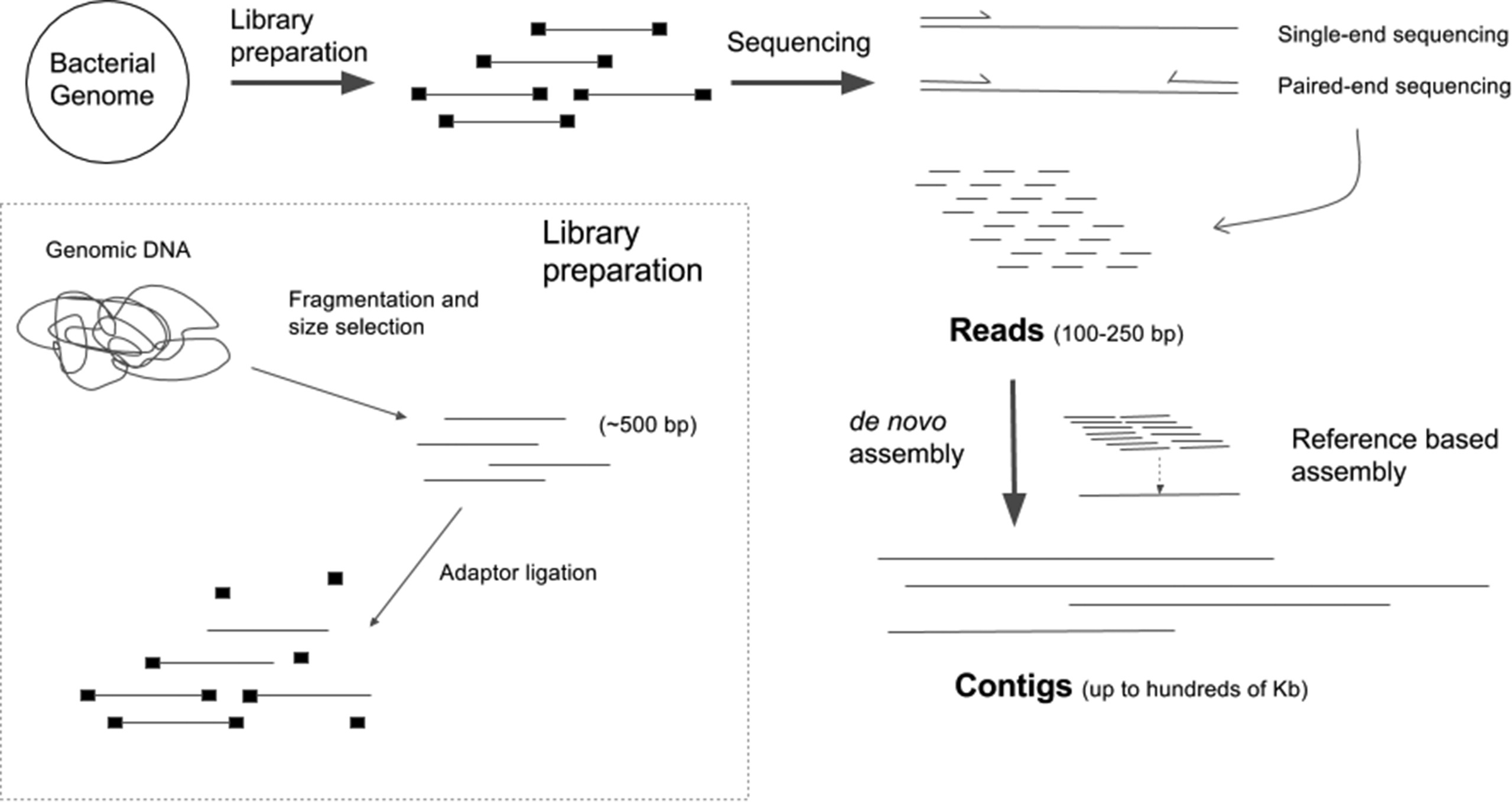
Sequencing Overview
Marker gene (16S, 18S, or ITS) is selected
Primers target areas of high conservation in gene
DNA is fragmented
Adapters are added to help the DNA attach to a flow cell
Barcodes may also be added to identify which DNA came from which sample
The fragments are sequenced to produce reads
Reads can be single-end (one strand sequenced) or paired-end (both strands sequenced)
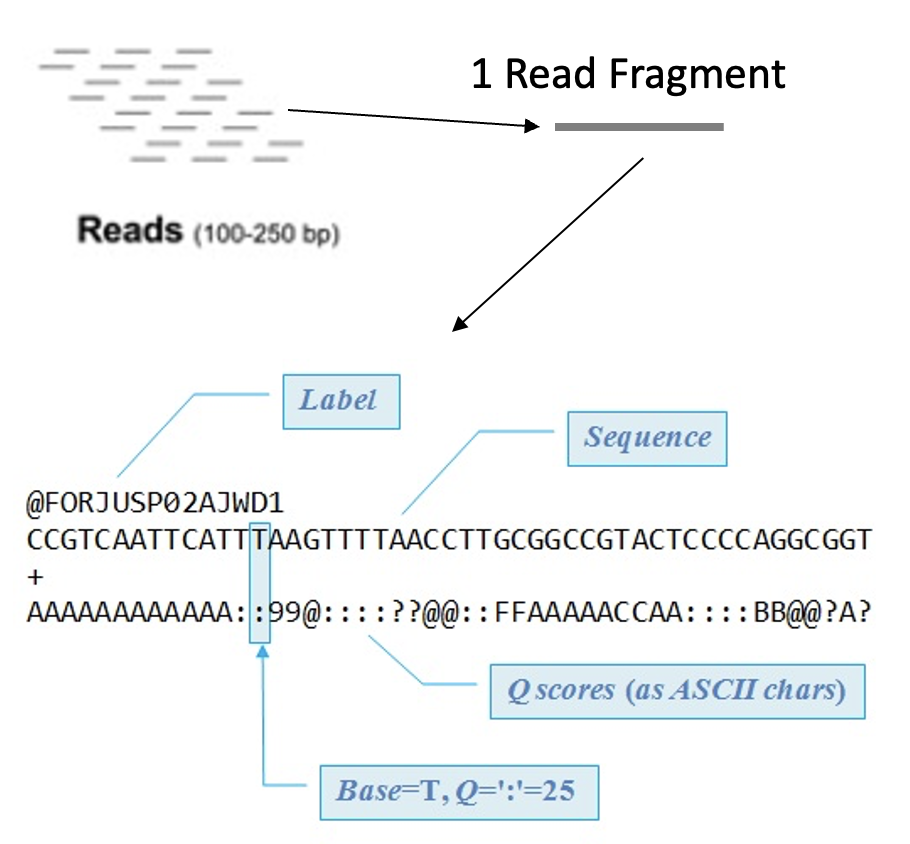
Sequencing Read Data
After sequencing we end up with a FASTQ file which contains:
A sequence label
The nucleic acid sequence
A separator
The quality score for each base pair
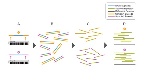
Demultiplexing
Sometimes samples are mixed to save on sequencing cost
To identify which DNA is from which sample Barcodes are added
Before moving forward samples need to separated and those DNA barcodes need to be removed
Tools like sabre can demultiplex pooled FASTQ data
Quality Scores
Quality Scores are the probability that a base was called in error
Higher scores indicate that the base is less likely to be incorrect
Lower scores indicate that the base is more likely to be incorrect
DADA2 Quality Control
Warning
DADA2 assumes that your read data has had any adapters removed and that your data is demultiplexed! Check out sabre to demultiplex your samples and Cutadapt to remove adapters.
We begin by specifying the path to our data, sorting by forward and reverse strands, and grabbing our sample names:
# path to files
path <- "../data/raw_fastq"

# sort our files by forward and reverse strands
# so that the sample names for each strand matches
# our data has the pattern "_pass_1.fastq.gz"
# and "_pass_2.fastq.gz"
path2Forward <- sort(
  list.files(
    path,
    pattern="_pass_1.fastq.gz",
    full.names = TRUE)
  )
path2Reverse <- sort(
  list.files(
    path,
    pattern="_pass_2.fastq.gz",
    full.names = TRUE)
  )

# now let's grab our sample names
sampleNames <- sapply(
  strsplit(
    basename(path2Forward), "_"), `[`, 1)
DADA2 has built in plotting features that allow you to inspect your fastq files:
# plot the forward strand quality plot of our first two sample
dada2::plotQualityProfile(path2Forward[1:2])+
  guides(scale = "none")

# plot the reverse strand quality plot of our first two sample
dada2::plotQualityProfile(path2Reverse[1:2])+
  guides(scale = "none")
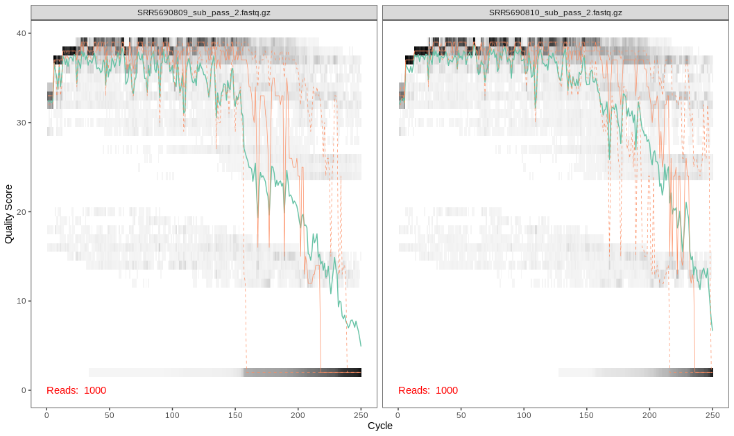
What does the graph tell us?
Here we see that the quality scores drop off around the 200th base position for the forward reads and the 150th base position for the reverse reads
The error rate is considered when determining true biological sequences but is more sensitive to rare biological senquences when reads are trimmed.
Trimming Considerations
The data we are using are 2x250 V4 sequence data. For data that do not overlap as much (i.e. data from the V1-V2 or V3-V4 regions), be wary that this may affect how the reads are merged later on.
Trimming
Here we notice a dip in quality scores and will trim using the base DADA2 filters:
# create new file names for filtered forward/reverse fastq files
# name each file name in the vector with the sample name
# this way we can compare the forward and reverse files
# when we filter and trim
filtForward <- file.path(path, "filtered", paste0(sampleNames, "_F_filt.fastq.gz"))
filtReverse <- file.path(path, "filtered", paste0(sampleNames, "_R_filt.fastq.gz"))
names(filtForward) <- sampleNames
names(filtReverse) <- sampleNames

# Now we will filter and trim our sequences
out <- filterAndTrim(
  path2Forward,
  filtForward,
  path2Reverse,
  filtReverse,
  truncLen = c(200,150),
  maxN=0,
  maxEE=c(2,2),
  truncQ=2,
  rm.phix=TRUE,
  compress=TRUE)