Differential Abundance
When assessing a microbial community, you might be interested to determine which taxa are differentially abundant between conditions. Given that we have a counts matrix we can use DESeq2!
Phylum Present
Before we assess which phylum are differentially abundant, a bar plot can be a quick first pass at determining this:
# transform the sample counts to proportions
# separate out our proportions
# separate our our tax info
ps.prop <- transform_sample_counts(ps, function(OTU) OTU/sum(OTU))
otu = data.frame(t(data.frame(ps.prop@otu_table)))
tax = data.frame(ps.prop@tax_table)

# merge the otu table and phylum column
# reshape our data to be accepted by ggplot
# merge taxa data with sample meta data
merged <- merge(otu,
                 tax %>% select(Phylum),
                 by="row.names") %>%
  select(-Row.names) %>%
  reshape2::melt() %>%
  merge(.,
        data.frame(ps.prop@sam_data) %>%
          select(Run,Host),
        by.x="variable",
        by.y="Run")

# plot our taxa
taxa_plot <- ggplot(merged,aes(x=variable,y=value,fill=Phylum)) +
  geom_bar(stat='identity') +
  theme_bw()+
  theme(axis.text.x = element_text(angle=45,hjust=1))+
  labs(
    x="",
    y="Abundance",
    title = "Barplot of Phylum Abundance"
  )+
  facet_wrap(Host ~ ., scales = "free_x")
taxa_plot
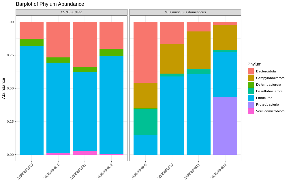
Here we note that the wild type seem to have an abundance of Campylobacteria and the C57BL/6NTac have an abundance of Bacteriodota. Let’s see if our DESeq2 results confirm this.
Differential Abundance
Differential Abundance measures which taxa are differentially abundant between conditions. So how does it work:
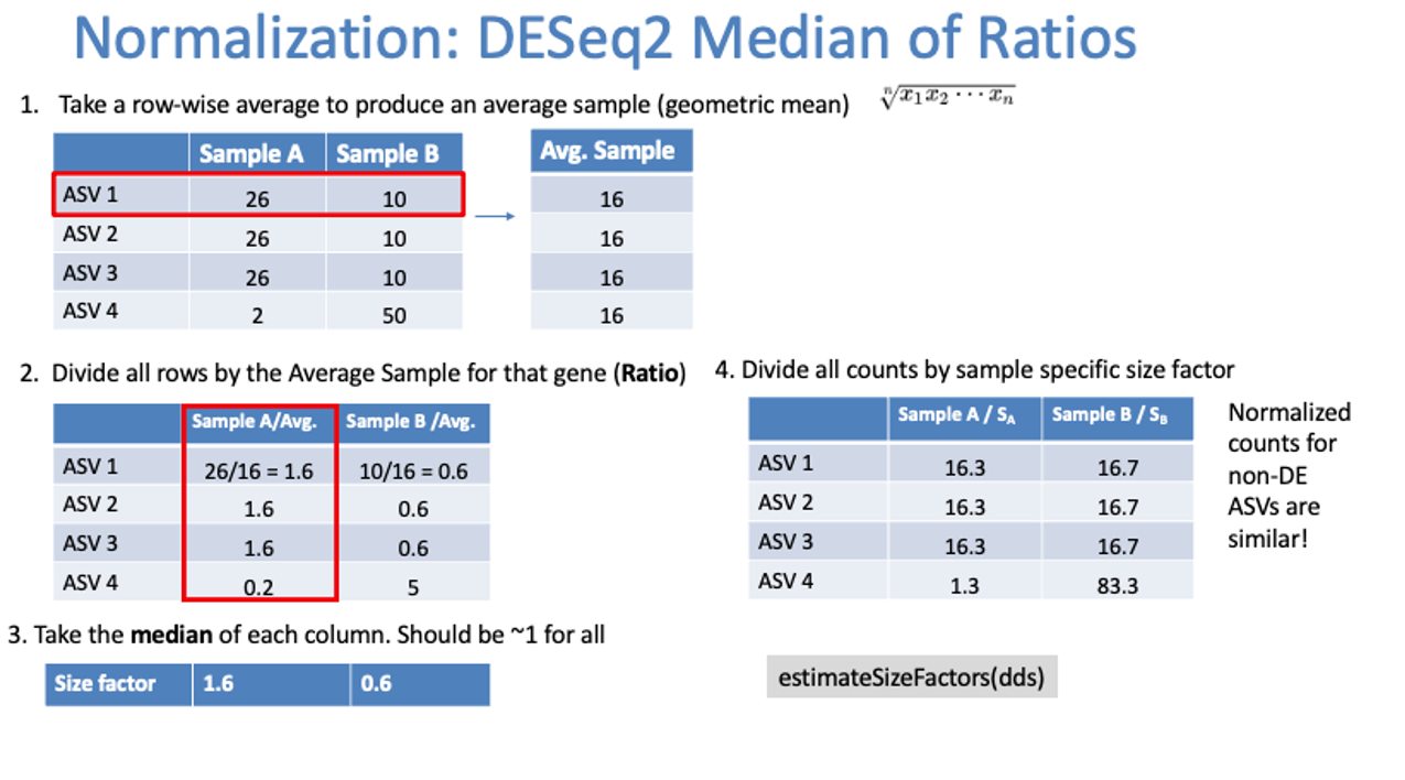
DESeq2 Normalization:
Geometric mean per ASV
Divide rows by geometric mean
Take the median of each sample
Divide all ASV counts by that median
DESeq2 Model
The normalized abundances of an ASV are plotted against two conditions
The regression line that connects these data is used to determine the p-value for differential abundance

DESeq2 P-Value
The Slope or 𝛽1 is used to calculate a Wald Test Statistic 𝑍
This statistic is compared to a normal distribution to determine the probability of getting that statistic

Now how do we do this in R?
# Differential Abundance

## convert phyloseq object to DESeq object this dataset was downsampled and
## as such contains zeros for each ASV, we will need to
## add a pseudocount of 1 to continue and ensure the data are still integers
## run DESeq2 against Host status, and ensure wild type is control,
## filter for significant changes and add in phylogenetic info
dds = phyloseq_to_deseq2(ps, ~ Host)
dds@assays@data@listData$counts = apply((dds@assays@data@listData$counts +1),2,as.integer)
dds = DESeq(dds, test="Wald", fitType="parametric")
res = data.frame(
  results(dds,
          cooksCutoff = FALSE,
          contrast = c("Host","C57BL/6NTac","Mus musculus domesticus")))
sigtab = res %>%
  cbind(tax_table(ps)[rownames(res), ]) %>%
  dplyr::filter(padj < 0.05)

## order sigtab in direction of fold change
sigtab <- sigtab %>%
  mutate(Phylum = factor(as.character(Phylum),
                        levels=names(sort(tapply(
                          sigtab$log2FoldChange,
                          sigtab$Phylum,
                          function(x) max(x)))))
  )

# as a reminder let's plot our abundance data again
taxa_plot

## plot differential abundance
ggplot(sigtab , aes(x=Phylum, y=log2FoldChange, color=padj)) +
  geom_point(size=6) +
  theme_bw() +
  theme(axis.text.x = element_text(angle = 60, hjust = 1)) +
  ggtitle("Mus musculus domesticus v. C57BL/6NTac")
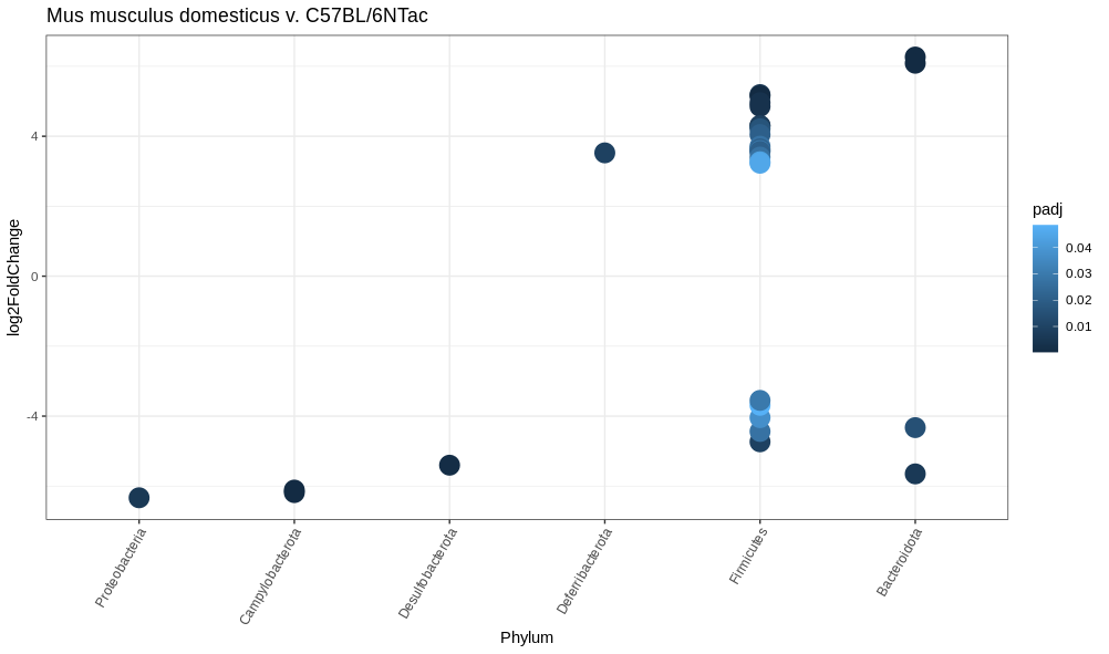
Explanation of Results
Wild type seem to have an abundance of Campylobacteria and the C57BL/6NTac have an abundance of Bacteriodota
Proteobacteria are severely downregulated in our C57BL/6NTac mice. However, they only show up in one sample!
Be sure that your data are not influenced by outliers!
Additionally, we collapsed our ASV’s to the Phylum level since all ASV’s had an identified phylum
References
A primer on microbial bioinformatics for nonbioinformaticians
DADA2: High resolution sample inference from Illumina amplicon data
Chimeric 16S rRNA sequence formation and detection in Sanger and 454-pyrosequenced PCR amplicons
Evaluation of 16S rRNA Databases for Taxonomic Assignments Using a Mock Community
Wild Mouse Gut Microbiota Promotes Host Fitness and Improves Disease Resistance
Normalization and microbial differential abundance strategies depend upon data characteristics
Waste Not, Want Not: Why Rarefying Microbiome Data Is Inadmissible
The neighbor-joining method: a new method for reconstructing phylogenetic trees.
Large-scale contamination of microbial isolate genomes by Illumina PhiX control